Usage
Installation
To install dive, install it with pip. Please note that the PyPI package name is
dive-EPR:
pip install dive-EPR
To use dive, import it as usual:
import dive
You should also import important modules such as:
import pymc as pm
import numpy as np
import matplotlib.pyplot as plt
import arviz as az
import deerlab as dl
from scipy.io import loadmat
Reading Data
If you already have experimental traces that you wish to analyze, load them in
as usual. Two example data files, 3992_good.dat and 3992_bad.dat, are
also included with dive in the /data folder.
For example,
# example data in /data
loaded_data = np.genfromtxt(f"data/3992_good.dat", skip_header=1, delimiter=',')
t = loaded_data[:,0]
Vexp = loaded_data[:,1]
If you would instead like to create synthetic data, follow this tutorial from DeerLab or use the built in functions at Reading & Creating Data.
Modeling
Next, you should create for PyMC to run numerical sampling with
dive.model. Detailed information can be found at Modeling.
# a shorter rmax is recommended for better and faster sampling
r = np.linspace(1.5, 6.5, 51)
# non-parametric (Tikhonov regularization):
model_tikh = dive.model(t, Vexp, method="regularization", r=r)
# parametric (Gaussian mixture model):
model_gauss = dive.model(t, Vexp, method="gaussian", n_gauss=2, r=r)
Sampling
You can now sample the model with PyMC through dive.sample. See
Sampling for more information.
# non-parametric
trace_tikh = dive.sample(model_tikh, draws=2000, tune=1000, chains=4, random_seed=101)
# parametric
trace_gauss = dive.sample(model_gauss, draws=2000, tune=1000, chains=4, random_seed=101)
The output of dive.sample is an
ArviZ InferenceData object.
Saving
The traces can be saved with dive.save_trace and dive.load_trace.
More information can be found at Saving.
dive.save_trace(trace_tikh, "data/example_trace_tikh")
dive.save_trace(trace_gauss, "data/example_trace_gauss")
trace_tikh, model_tikh = dive.load_trace("data/example_trace_tikh.nc")
trace_gauss, model_gauss = dive.load_trace("data/example_trace_gauss.nc")
Validating
Before moving on to data analysis, it is important to make sure that the chains are stable and converged. Below are a few functions that are helpful in assessing chain convergence and quality:
dive.print_summary(trace): This prints a data table containing information
about the marginalized parameter distributions, including their mean,
94% confidence interval, skewness, etc. For validating our results, however,
we are most interested in the rightmost column titled r_hat.
r_hat is the ratio of interchain variance to intrachain variance.
If it is close to 1, then the variances are similar, meaning that the chains
have converged to similar regions.
r_hat values below 1.05 suggest good convergence, and it is encouraged
that the r_hat for every variable in dive.print_summary should be below
this value before you continue to analysis. (If you are just testing things out,
it is okay, though not ideal, to have higher values of r_hat.)
Documentation can be found in Plotting.
dive.print_summary(trace_tikh)
dive.print_summary(trace_gauss)
                    mean    sd          hdi_3%      hdi_97% mcse_mean       mcse_sd ess_bulk        ess_tail        r_hat
$λ$                     0.533       0.007   0.521   0.546   0.000       0.000       1040.0      1656.0          1.01
$V_0$                   1.007       0.010   0.990   1.026   0.000       0.000       1819.0      3126.0          1.00
$σ$                     0.021       0.001   0.019   0.023   0.000       0.000       4447.0      3908.0          1.00
$\mathrm{lg}(α)$    -0.462  0.074   -0.597  -0.322  0.002       0.001       2225.0      3735.0          1.00
$B_\mathrm{end}$    0.897   0.015   0.872   0.929   0.000       0.000       1390.0      970.0           1.01
                    mean    sd      hdi_3%  hdi_97%         mcse_mean       mcse_sd ess_bulk        ess_tail        r_hat
$λ$                     0.502       0.005   0.495   0.512   0.001       0.001       16.0        70.0            1.19
$V_0$                   0.977       0.007   0.963   0.991   0.001       0.001       33.0        191.0           1.14
$σ$                     0.021       0.001   0.019   0.022   0.000       0.000       12.0        21.0            1.39
$r_{0,1}$           3.337   0.571   2.156   3.849   0.185       0.142       7.0         123.0           1.56
$r_{0,2}$           3.989   0.076   3.911   4.123   0.037       0.028       5.0         16.0            2.03
$w_1$                   1.157       0.908   0.348   2.998   0.265       0.192       16.0        128.0           1.32
$w_2$                   0.494       0.108   0.282   0.603   0.052       0.040       6.0         14.0            1.77
$a_1$                   0.264       0.259   0.001   0.708   0.126       0.097       6.0         51.0            1.91
$a_2$                   0.736       0.259   0.292   0.999   0.126       0.096       6.0         49.0            1.91
$B_\mathrm{end}$    0.850   0.009   0.839   0.866   0.002       0.002       14.0        134.0           1.21
az.plot_trace(trace): This helpful function from the arviz library makes
two plots for each parameter. On the left, it plots the marginalized posterior
of the parameter for each chain (if you set combined to False). This is
very helpful in visualizing convergence. If you see one (or more) chains with a
significantly different posterior plot, it is like unconverged. On the right,
it plots the value of the parameter chronologically for each chain.
If you notice that it gets ‘stuck’ (showing the same value for many draws in a
row), it may be sampling poorly.
See the documentation for az.plot_trace.
# non-parametric trace is converged:
az.plot_trace(trace_tikh, var_names=["lamb","Bend","V0","sigma","lg_alpha"], combined=False)
# parametric trace is not converged
az.plot_trace(trace_gauss, var_names=["lamb","Bend","V0","sigma","r0","w","a"], combined=False)
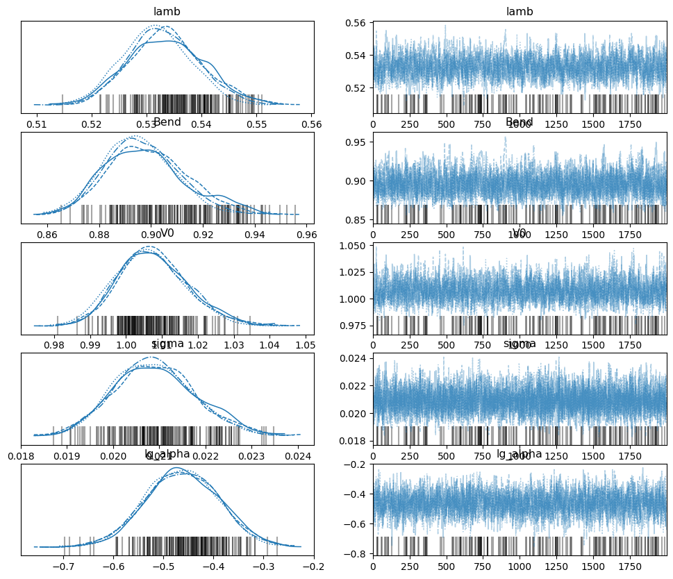
It can be seen that the non-parametric trace is well-converged, while the
parametric trace is not. This is probably because the sampler does not know
where to put the second gaussian in the parametric trace, as shown by the large
uncertainties in its mean (r0), width (w), and amplitude (a) on the
arviz plot. Changing the model to be a 1-gaussian model would likely help with
convergence.
Question: My chains aren’t converged! What should I do?
Answer: Try the following steps:
1. Increase the number of draws. Most often, you just need to run your trace for longer to attain convergence.
2. Increase the number of tunes. Proper tuning is important to good sampling, and increasing the number of tuning steps may help, though anything above 2000 tunes per chain probably will not be too helpful.
3. Adjust your model. For example, shortening the maximum value of the r-axis will lead to faster sampling and convergence. You may also want to consider changing the number of gaussians (if using a parametric model) and changing the resolution of the r-axis.
4. Prune chain(s). If you notice that one (or more) chains are particularly
unconverged, but the rest are decent, then you could remove the faulty chain(s).
You can do this through dive.prune_chains(trace), which drops each chain one
by one and pruning the one that reduces r_hat the most, repeating until
converged. You can also remove chains with
trace.sel(chain=desired_chain_numbers). Note that pruning chains will not be
very effective if all of your chains are very different from each other.
5. Set alpha to a fixed value. This can be done by passing an alpha
parameter in dive.model(). Removing a parameter may make for better
sampling. However, fixing a parameter will also limit the validity of the
uncertainty analysis, so do this with caution.
Accessing Results
The output of dive.sample is an ArviZ InferenceData object
that consists of three xarray objects: posterior, sample_stats, and
observed_data.
We are primarily interested in trace.posterior, which is an xarray object
containing all of our parameters as data variables, the chains and draws as
coordinates, and some supplementary information as attributes.
print(trace_tikh.posterior)
<xarray.Dataset> Size: 7MB
Dimensions:            (chain: 4, draw: 2000, P_dim_0: 51, P_Dirichlet_dim_0: 51)
Coordinates:
* chain              (chain) int64 32B 0 1 2 3
* draw               (draw) int64 16kB 0 1 2 3 4 ... 1995 1996 1997 1998 1999
* P_Dirichlet_dim_0  (P_Dirichlet_dim_0) int64 408B 0 1 2 3 4 ... 47 48 49 50
* P_dim_0            (P_dim_0) float64 408B 1.5 1.6 1.7 1.8 ... 6.3 6.4 6.5
Data variables:
    Bend               (chain, draw) float64 64kB 0.8891 0.8917 ... 0.8683
    P                  (chain, draw, P_dim_0) float64 3MB ...
    P_Dirichlet        (chain, draw, P_Dirichlet_dim_0) float64 3MB ...
    V0                 (chain, draw) float64 64kB 1.003 0.9967 ... 1.003 1.01
    delta              (chain, draw) float64 64kB ...
    k                  (chain, draw) float64 64kB ...
    lamb               (chain, draw) float64 64kB 0.5271 0.5239 ... 0.5251
    lg_alpha           (chain, draw) float64 64kB -0.4515 -0.4756 ... -0.6419
    lg_delta           (chain, draw) float64 64kB ...
    sigma              (chain, draw) float64 64kB 0.01939 0.02025 ... 0.02026
    tau                (chain, draw) float64 64kB ...
Attributes: (12/14)
    created_at:                 2024-08-06T20:39:37.362330+00:00
    arviz_version:              0.18.0
    inference_library:          pymc
    inference_library_version:  5.10.4
    sampling_time:              519.4337060451508
    tuning_steps:               1000
    ...                         ...
    include_background:         1
    include_mod_depth:          1
    include_amplitude:          1
    delta_prior:                [1.e+00 1.e-06]
    tau_prior:                  [1.e+00 1.e-04]
    random_seed:                101
The array stores the values for each parameter in the order they were generated,
so if we wanted to find the value of lamb for the first draw of the first
chain, we would print:
print(trace_tikh.posterior.lamb[0][0])
<xarray.DataArray 'lamb' ()> Size: 8B
array(0.527104)
Coordinates:
    chain    int64 8B 0
    draw     int64 8B 0
Oftentimes, however, this is not a very convenient way to access the posterior
distributions. Instead, we can use the function az.extract,
which allows us to extract the parameters we want and stack them to combine the
chain and draw dimensions.
import arviz as az
lamb_array = az.extract(trace_tikh, var_names=["lamb"]) # extracts all the value of lambda for all samples and stacks them
print(lamb_array.values) #.values converts the xarray into a numpy array
[0.52710417 0.52392079 0.53517045 ... 0.53273982 0.53126788 0.52509982]
With an xarray/numpy array of your parameters, you can perform your data analysis as usual. ArviZ may also have useful functions for data analysis, including az.hdi, which calculates the highest density interval (the equivalent of a confidence interval) for some parameter.
lamb_hdi = az.hdi(trace_tikh, hdi_prob=0.95, var_names=["lamb"]) # calculates the 95% highest density interval for lambda
print(lamb_hdi)
<xarray.Dataset> Size: 64B
Dimensions:  (hdi: 2)
Coordinates:
* hdi      (hdi) <U6 48B 'lower' 'higher'
Data variables:
    lamb     (hdi) float64 16B 0.5202 0.5457
More information about InferenceData objects can be found here.
Plotting
dive provides several useful plots for assessing fit and investigating
marginalized posterior distributions. Please see Plotting for full
documentation. A few funcitons are outlined below:
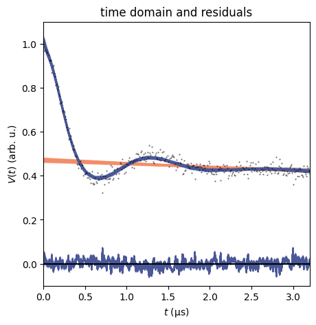
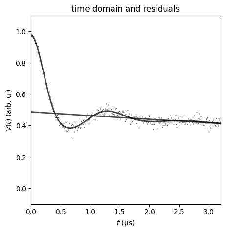
dive.plot_V plots an ensemble of modelled signals to the true signal,
along with residuals and a corresponding ensemble of background fits.
dive.plot_V(trace_tikh)
dive.plot_V(trace_gauss,show_avg=True,hdi=0.95)
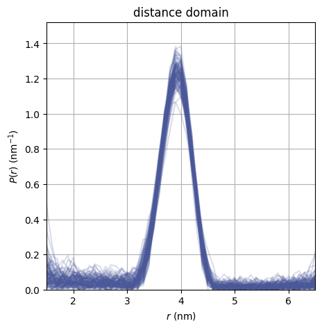
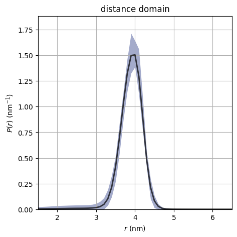
dive.plot_P plots an ensemble of distance distributions to give a
visualization of the uncertainty of P.
dive.plot_P(trace_tikh)
dive.plot_P(trace_gauss,show_avg=True,hdi=0.95,alpha=0.5)
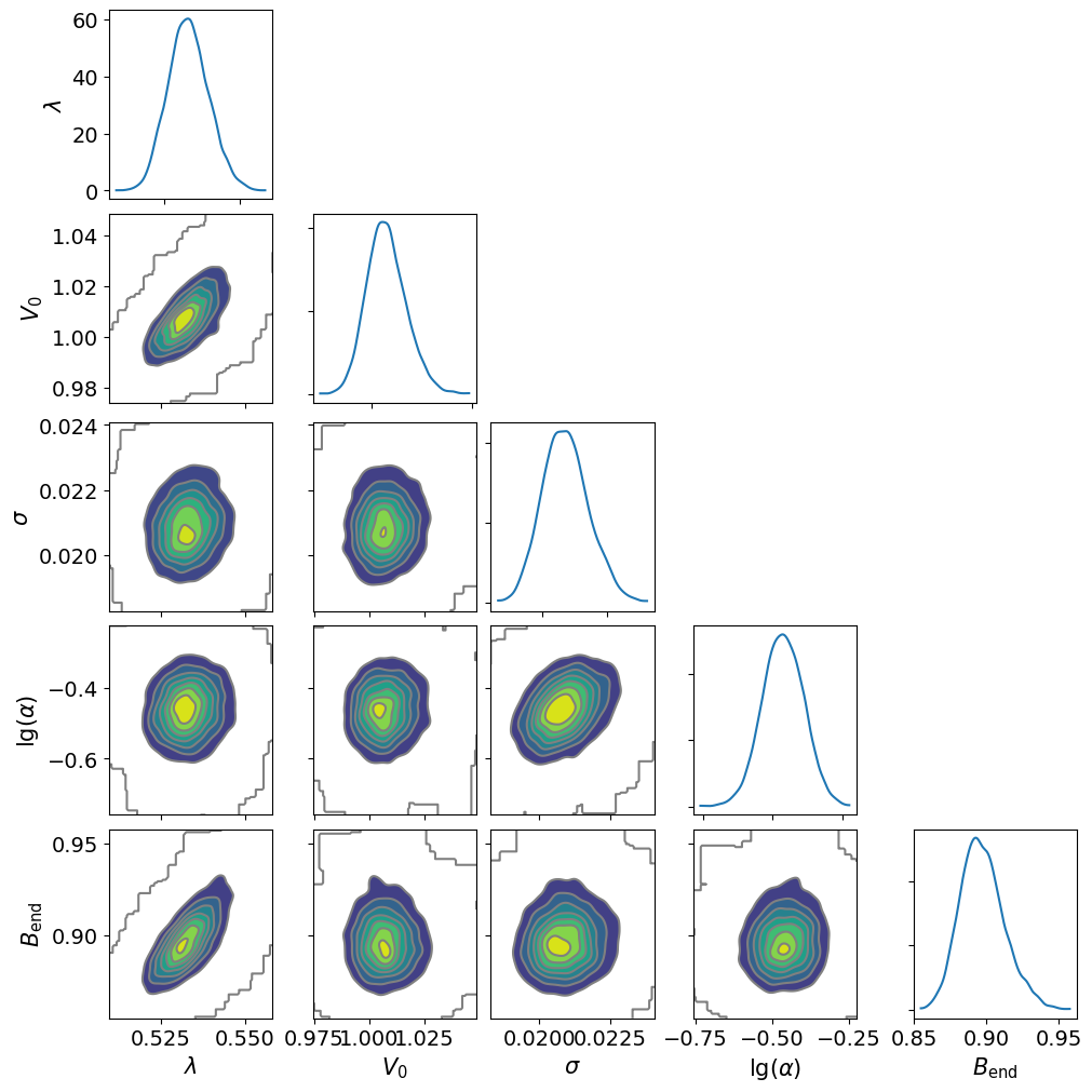
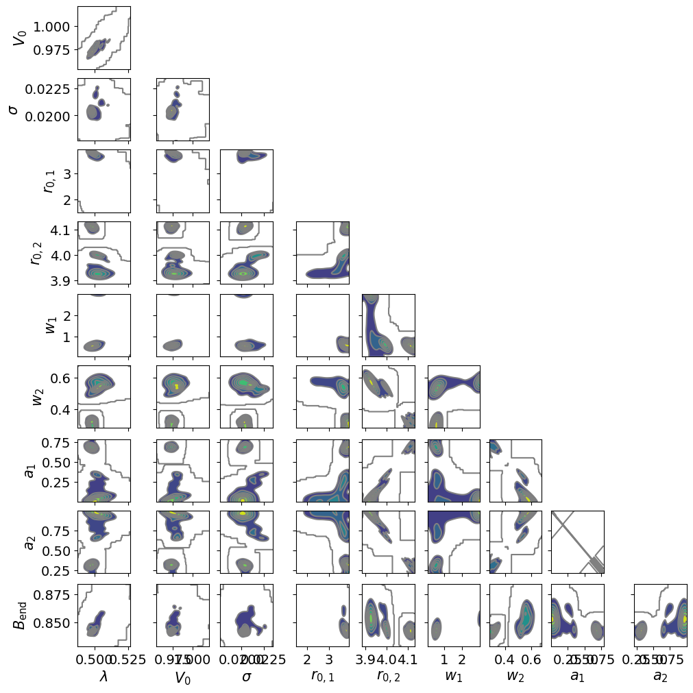
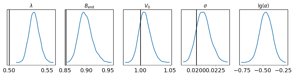
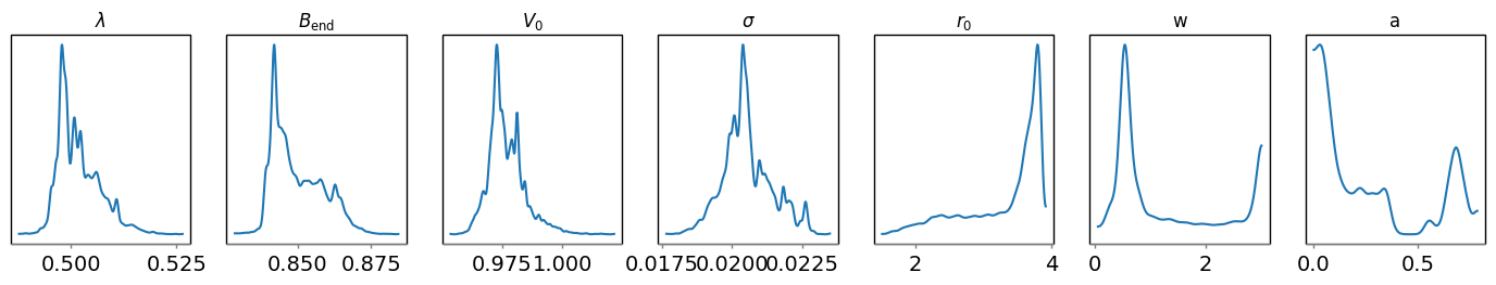
For the marginal posteriors of the other parameters, you can call
dive.plot_marginals for 1D marginalized distributions and
dive.plot_correlations for 2D marginalized distributions.
dive.plot_marginals(trace_tikh, var_names=["lamb","Bend","V0","sigma","lg_alpha"], ground_truth={"lamb":0.5,"Bend":np.exp(-0.05*3.2),"V0":1,"sigma":0.02})
dive.plot_marginals(trace_gauss, var_names=["lamb","Bend","V0","sigma","r0","w","a"]) # spiky/uneven plots due to poor convergence
dive.plot_correlations(trace_tikh)
dive.plot_correlations(trace_gauss,marginals=False)